Introduction

This blog post describes a custom R implementation and a backtest analysis of the Markowitz Global Minimum Variance (GMV) portfolio allocation strategy.  In this post, we utilize a simple quadratic solver to perform the necessary optimizations and subsequently execute our backtests on historical data of two distinct portfolios:

• the SPDR exchange traded funds.
• A subset of the stocks that are currently included in the benchmark stock market index of Euronext Brussels (BEL20)

It should be noted that it is well known that the Markowitz portfolio allocation model returns suboptimal results due to its underlying normality assumptions and its inability to robustify against parameter estimation errors and model uncertainty. Hence, this post serves as an introduction to more involved portfolio optimization techniques that take these issues into account in future posts.

The accompanied source code can be retrieved from this Github repository.

Markowitz and the Efficient Frontier

According to Markowitz, investors should perform portfolio allocations based upon on a trade-off between risk and expected returns of the assets under consideration. Expected returns are defined as the expected future price changes (including additional income such as dividends) divided by the current starting prices of the securities. On the other hand, risk should be measured by the variance of the returns, which is defined as the average squared deviation around the expected returns.

Moreover, Markowitz argued that for any given level of expected portfolio return, a rational investor would choose the portfolio with minimum variance between the set of all possible portfolios. The set of possible portfolios is called the feasible set and the minimum variance portfolios are called the Mean-Variance efficient portfolios. The set of all mean-variance efficient portolios for different desired levels of expected return is called the efficient frontier. View the image in the sideline below for some additional insight.

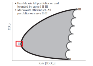
Curve II-III represents the portfolios on the efficient frontier. These portfolios offer the lowest level of standard deviation (and variance) for a given level of expected return. In this article we focus on the portfolio at point II, which is referred to as the global minimum variance (GMV) portfolio. It is the portfolio on the efficient frontier with the smallest overall variance.

Mathematical Formulation of Markowitz and GMV Portfolios

Let’s suppose that an investor has a choice between $latex N$ risky assets. This choice is represented by an $latex N$-vector of weights $latex w =  (w_{1}, w_{2}, …, w_{N})^T$, where each weight i represents the percentage of the i-th asset held in the portfolio, and hence

$latex \sum_{i=1}^{N}w_{i} = 1$

Now, let’s assume that the asset returns $latex \textbf{R} = (R_{1}, R_{2}, …, R_{N})^T$ have expected returns $latex \boldsymbol\mu = (\mu_{1}, \mu_{2}, …, \mu_{N})^T $ and the $latex N \times N$ covariance matrix between the returns is given by:

$latex \boldsymbol\Sigma = \begin{pmatrix} \sigma_{11} & … & \sigma_{1N} \\ .. & .. & .. \\ \sigma_{N1} & … & \sigma_{NN} \end{pmatrix} $

where $latex \sigma_{ij}$ denotes the covariance between asset i and asset j such that $latex \sigma_{ii} = \sigma_{i}^{2}, \sigma_{ij} = \rho_{ij}\sigma_{i}\sigma_{j}$ and $latex \rho_{ij}$ represents the correlation between asset i and asset j. Under these assumptions, the return of a portfolio with weights $latex w = (w_{1}, w_{2}, …, w_{N})^T$ is a random variable $latex R_{\rho} = \mathbf{w^TR}$ with expected return and variance given by

$latex \mu_{\rho} = \mathbf{w^T}\boldsymbol\mu$

$latex \sigma_{\rho}^{2} = \mathbf{w^T}\boldsymbol\Sigma\mathbf{w}$

Note that by choosing the portfolio weights, an investor effectively chooses between the available mean-variance pairs. To calculate the weights for one possible pair, we choose a target mean return, $latex \mu_{0}$. If we follow Markowitz reasoning -as explained in the previous paragraph- the investment problem expresses itself as a constrained minimization problem in the sense that the investor must seek

$latex \min\limits_{w} \mathbf{w^T}\boldsymbol\Sigma\mathbf{w}$

subject to the constraints

$latex \mu_{0} = \mathbf{w^T}\boldsymbol\mu$

$latex \mathbf{w^T}\boldsymbol\iota = 1, \boldsymbol\iota^T = [1, 1, …, 1]$

This problem expresses itself as a rather simple quadratic optimization problem with two equality constraints. Furthermore, as we already mentioned, in this article we are only interested in the GMV portfolio (point II on the efficient frontier in the above image). This implies that the problem can be further simplified by removing the first equality constraint from the formulation. In other words, we want to obtain the portfolio that obtains minimum variance without taking the associated expected portfolio return into account.

R Demo

In this section we backtest a GMV portfolio strategy on two distinct portfolios. The associated source code is hosted on Github. The reader can replicate the analysis and results locally by running the demo.R script.

Assets Under Consideration

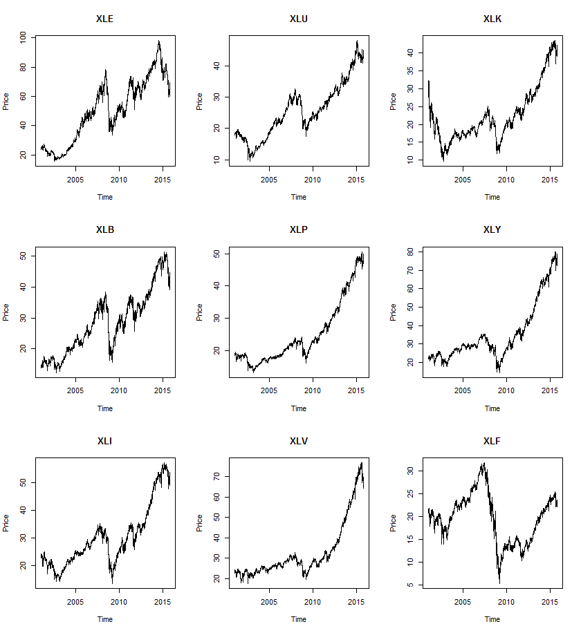
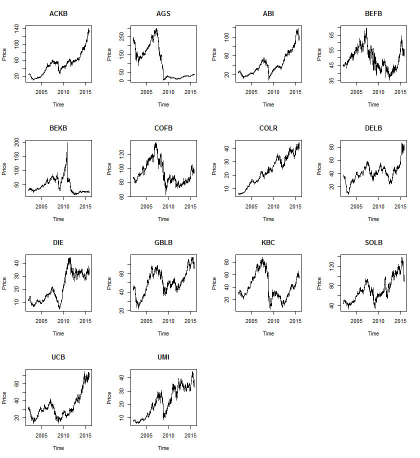
In this article, we consider the historical backadjusted openingprices of the SPDR ETF funds and 14 of the stocks underlying the BEL20 index. Note that backadjusted prices account for dividends, mergers and stock splits in such a way that the associated asset returns include all the required information. The code snippet below loads the provided SPDR asset data into an xts timeseries object. The asset returns are subsequently calculated and a graphical representation of the historical stock prices is generated.

The images below illustrate the historical backadjusted stock prices of the underlying assets for both portfolios under consideration.

Converting the GMV Formulation into a Quadratic Program

We use the solve.QP function from the quadprog package to solve the GMV quadratic programming problem. The solve.QP routine implements the dual method of Goldfarb and Idnani (1983) for solving problems of the following form:

$latex \min\limits_{x} -d^Tx + \frac{1}{2} x^TDx $

subject to the following constraints

$latex A^Tx \geq b_{0}$

The required arguments of the function can be obtained from the package documentation. The arguments and their descriptions are copied below for the readers convenience:

• Dmat – matrix appearing in the quadratic function to be minimized.
• dvec – vector appearing in the quadratic function to be minimized.
• Amat – matrix defining the constraints under which we want to minimize the quadratic function.
• bvec – vector holding the values of $latex b_{0}$ (defaults to zero).
• meq – the first meq constraints are treated as equality constraints, all further as inequality constraints (defaults to 0).
• factorized – logical flag: if TRUE, then we are passing R^(-1) (where D = R^T R) instead of the matrix D in the argument Dmat.

Custom GMV Implementation

The implementation of the GMV optimization procedure is illustrated in the code snippet below. However, we added a few additional tweaks: Note that the original GMV formulation allows for short positions (negative asset weights) and relatively unrestricted asset weight proportions. In our custom implementation we allow the users to specify an optional longOnly flag and we give them the possibility to set a maximum weight allocation for individual assets. The latter condition implies that the absolute values of the individual asset weights must be smaller than max.weight.

We further note that the procedure expects an xts object containing the asset return timeseries as input in order to calculate the covariance. The procedure returns the requested GMV weights that are associated with the input settings:

Backtesting the GMV Portfolio Strategy

In this section we perform an out of sample backtest of the GMV portfolio strategy that was implemented in the section above. The goal here is to first obtain the GMV weights for the available historical timestamps and subsequently compare the resulting portfolio allocations with the actual next-day realized returns of the assets. The out of sample results can then be plotted and analyzed. Furthermore, we also need to define an additional lookback setting to indicate how much historical data we want to use for our covariance matrix calculation. It is important to note that we can only look at the data that is already available to us on any given timestamp in order to avoid any potential data-snooping bias.

The backtest function is added in the code snippet below. Note that the procedure uses the foreach package to run the optimizations in parallel across multiple CPU’s:

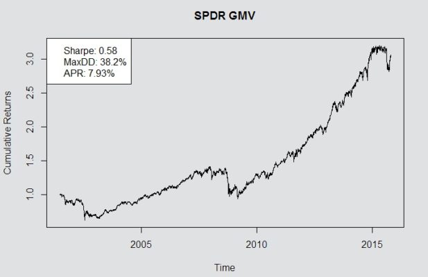
Demo Results

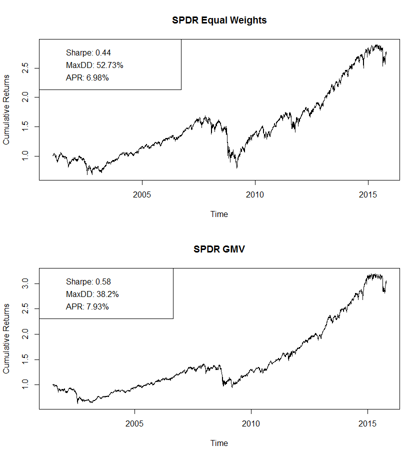
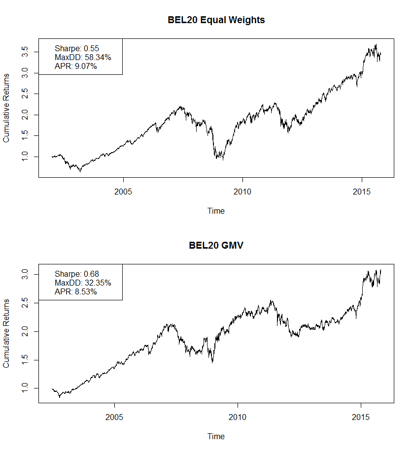
The github repository associated with this post contains a few plotting and performance metric functions that can be used to analyze the results further. Here, we compare the GMV strategy results with the corresponding equal weight allocation strategy. The GMV strategy demo settings are chosen ad hoc. The code snippet from the SPDR demo is added below for illustration purposes:

The results of the portfolio-strategy combinations are illustrated in the images below: